If you’ve been watching the news lately, you’ve likely seen a great deal of supply chain issues pop up. In the years leading up to the pandemic, the world’s supply chains functioned like a well-oiled machine. However, the flaws of global integration quickly took over when the pandemic hit.
In this new series of articles, I’ll cover some of the basic supply chain theories from my Supply Chain Management course at LSE. In part 1 we’ll work towards the Economic Order Quantity, a formula that allows you how many units you should order from your supplier.
Setting the stage
Let’s start by defining some assumptions.
The quantity we order each time is Q. We face demand from our customers of D units per year. And we pay an average price of C per unit. Whenever we place an order with our supplier, we pay a fixed fee of S. Lastly, holding a unit in our inventory also costs us money, H/unit/year. H can also be defined as a % of the unit price (h), such that H = h*C.
An overview:
- Q: quantity in a lot/batch/order
- D: demand (usually annualized)
- C: the average price paid per unit purchased
- S: a fixed cost you have to pay every time you order
- H: holding costs per unit
(usually annualized, matching the time period of D) - h: the holding cost as a % of unit cost (C)→ hC = H
Our inventory
Because we assume demand (D) is stable and that our suppliers deliver the second we place an order (”lead time” is zero), our inventory will look like a zigzag pattern.
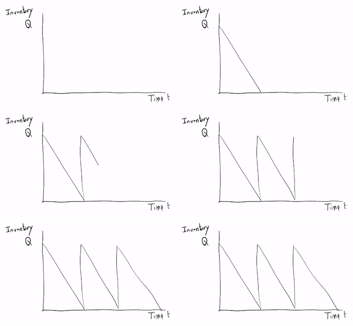
*What is the average inventory we hold (also known as the cycle inventory)?*→ In this case, it’s Q/2, the middle between the maximum and minimum.
This will be useful later when we calculate the holding cost of our inventory.
How long does a unit remain in our inventory on average?(also called “average flow time”)
→ If we assume a lot size (Q) of 1000, and a daily demand of 100, then the average unit would be in our inventory for (Q/2)/D days, or the cycle inventory divided by demand.
So why do we want a cycle inventory? Well, it has a few reasons. The first is that we can order in larger quantities, meaning that we can take advantage of economies of scale. And it means we are able to reduce costs, for example, transport is cheaper per “full truck load” (FTL).
Why not hold a huge cycle inventory? Doing so would be very capital intensive because you already paid for these units and it may take a while before you see your cash back. Capital is not free and could be invested elsewhere. Holding inventory is also not free, you may need a larger warehouse, better insurance, etc.
What does it cost?
To figure out what the optimal order quantity (“economic order quantity”, EOQ) is we need to specify the total annual cost.
Using this simple model we can define the following cost items:
The material cost is simply the number of units we handle in a year (the demand) multiplied by the unit cost. Orders per year is the demand divided by the quantity per order. The ordering cost (the fixed part) is just the cost per order multiplied by the order per year.
Finally, holding costs are the holding cost per unit multiplied by the cycle inventory (that we saw before).
Okay, let’s optimize these costs by looking at how they vary when we increase the order size (Q).
Material cost
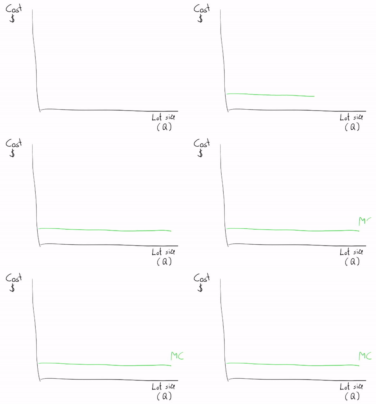
Material costs only depend on the annual demand and do not change with the order size (the formula is C*D, independent of Q).
Ordering cost
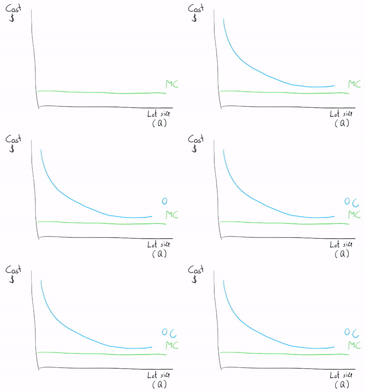
Ordering costs are inversely related to the order size. Ordering more at once means fewer orders. Because ordering costs are fixed per order the total will decrease if you make fewer orders.
Holding cost
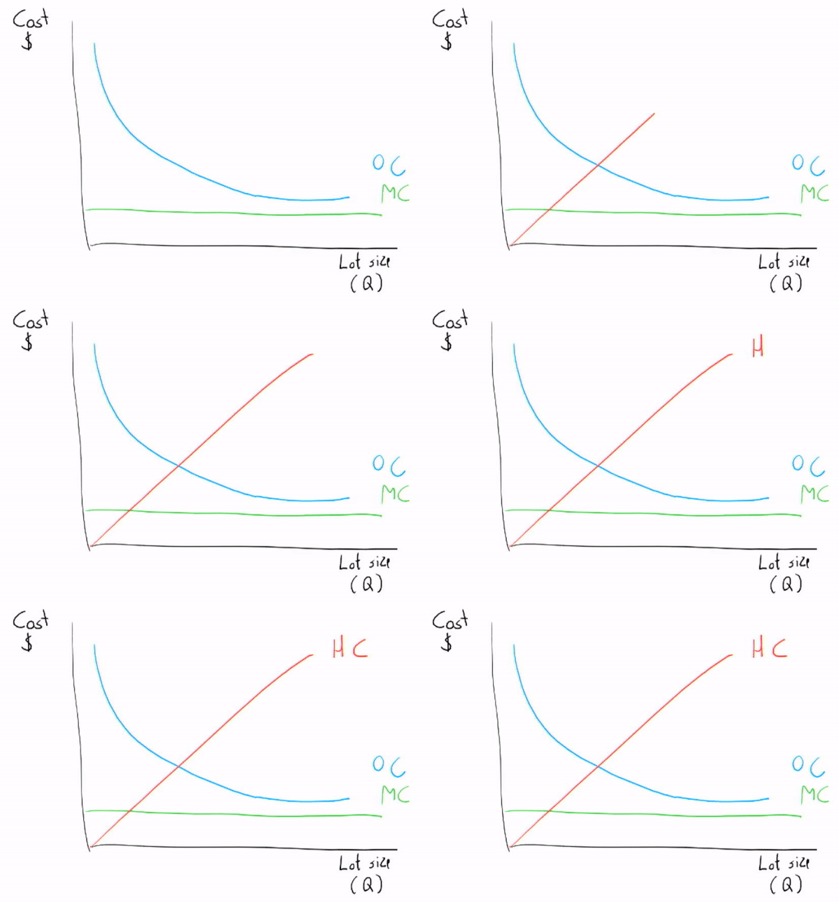
Holding cost increases in the lot size. If we order a unit with our supplier whenever we have a unit of demand, we have zero holding costs. In the real world this is the concept of drop shipping.
If we order large quantities we’ll need a large warehouse, lots of capital, etc. which are all very costly.
Total cost & the optimal lot size
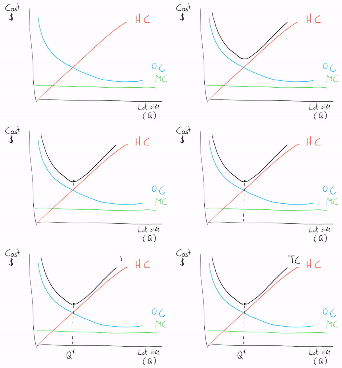
Total cost is simply the sum of all the lines. The optimal order size is found at the minimum of this line. Ordering at Q* means that your total annual cost is as low as it can possibly be.
If you’re into mathematics, Q* is where the first derivative of the total cost (TC) line is equal to zero. I’ll spare you the derivation but to find Q* in our model we can use the following formula:
Economic Order Quantity (EOQ)

Tying it all together
Now that we’ve seen a simple supply chain model, what can we say about reality?
Well, we know that without any uncertainty, the quantity ordered largely depends on how costly it is to hold inventory and what it costs to order a single lot.
Now imagine large deviations in demand, or the time it takes to receive goods (lead times), both of which happened during the pandemic. These are not considered in this model.
Companies anticipated a large drop in demand but we ended up seeing a V-shaped recovery in many sectors, with some seeing insane growth (and decline) due to changes in behavior.
Normally holding a large inventory would have been bad. With demand stagnating it could have taken companies years to get rid of their inventory, tying up the cash needed to survive a crisis. So companies canceled orders, entering survival mode. However, when demand spiked soon after, firms were left scrambling for inventory. Producers who had already scaled down production capacity could not keep up with demand, causing increased prices, order costs, and leading to shortages.
TL;DR
Under a stable demand you pick your optimal units per order through the economic order quantity formula (EOQ):

During the early days of the pandemic, we saw firms anticipate an economic downturn (less demand), canceling orders and entering survival mode (focusing on liquidity, cash).
When sectors saw demand spike (for example the semiconductor industry), inventories were low and production had been scaled down. Though firms had optimized for holding costs, they were now struggling with increased order costs and demand.
