
Many industries face seasonal demand in some form or another. On a monthly, quarterly, or even weekly basis, seasonality is everywhere. Because my Supply Chain Management course at the London School of Economics covered it recently, and I had applied it professionally before, I decided to create a quick guide for a static method.
Introduction
Put simply, a static seasonal forecasting model has three components:
- A level of demand that’s assumed to be the “base” (for those into statistics: the intercept)
- A trend that indicates the change in demand per period of time (the slope)
- A seasonal factor that can either be additive or multiplicative (more on that later)
Many guides will give you a bunch of formulas which is great if you want to know more about the theory, but here I’ll focus on an intuitive approach. If you do want to learn more I’ll leave the (more technical) resources at the end.
This method estimates a model for a given dataset, which can be based on a long history. It does not assign weights to more recent observations the way adaptive models would (like Holt-Winters). I will cover such a model in the near future, follow/subscribe to be notified when I do.
I will now go over the steps to build a static forecasting model:
- Get data and deseasonalize it.
- Estimate: a regression of deseasonalized demand on time to get level (intercept) and trend (slope).
- Estimate seasonal factors.
- Forecast.
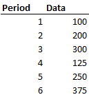
If you want to follow along you can use the following data:
Step 1: Deseasonalize it
Look at your data and determine your periodicity, i.e. after how many periods (days, weeks, months) does the pattern repeat itself? We’ll assign this the letter p. Plotting your data can help:
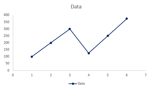
Here the pattern repeats every 3 periods (p = 3).
Now that we know our periodicity (p) we can apply a deseasonalizing formula (don’t worry I’ll explain it intuitively):
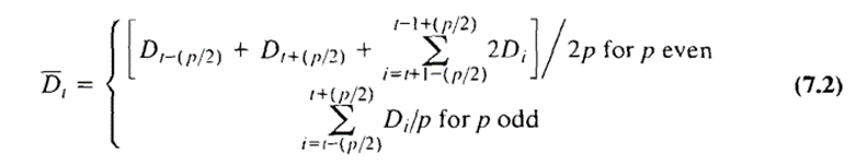
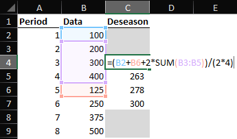
Because our p is odd we use the bottom formula. I’ll go over an example for an even p in the next section. The bottom formula is a fancy way of writing an average. In Excel, we can simply take the average over the range from t-(p/2) to t+(p/2). Here that’s from t-1 to t+1.
Another way to think about it: in every period, deseasonalized data should capture all seasons. Here there’s a low period, medium period, and high period of demand which are all equally weighted in the average.
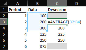
Note: the formula will not work for the first and last p/2 periods. In this case, periods 1 and 6. Due to the lack of data, you cannot look back/ahead.
For an even periodicity (p = 4)
For similar data that shows a periodicity of 4, we have to use the more complicated formula. Essentially, we take a weighted average with a greater weight on observations closer to us.
There are various technical reasons why this formula is the way it is. That’s beyond the scope of this article, I’ve linked a book chapter below in case you’re interested.
Step 2: Regress it
Using our p=3 data, run a regression of the deseasonalized data on time to get the level and trend.
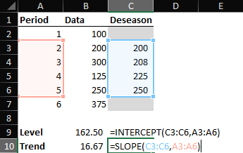
This can be seen as the underlying base level of demand and the trend in the underlying demand, without taking into account any seasonality. We’ll use this in our forecasting step.
Step 3: Get seasonal factors
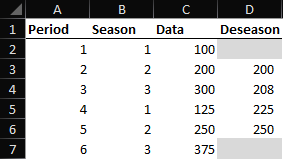
Seasonal factors can be modeled in an additive (absolute) or multiplicative (relative) way. Before we look at both ways we have to label the periodicity of our data. In some cases, you may already have this (e.g., your periodicity is 12 months and you have the months of the year).
Here I introduce a Season column that indicates the season of that period (and repeats after 3 periods, in line with our periodicity (p) of 3).
Additive
For the additive approach, the seasonal “factor ” is an absolute amount of demand that’s added or subtracted based on the season. We estimate this by taking the difference between the observed demand (Data) and our underlying demand (Deseason).
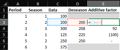
The additive approach is useful when the absolute seasonal effect does not change over time. I.e. the differences don’t scale proportional to demand but are fixed.
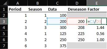
Multiplicative
When differences do scale with demand, using a multiplicative approach is better as it captures this “relative” seasonality. To find the multiplicative factor, simply divide actual demand by the deseasonalized one.
Averaging the factors
Here, season 2 has a seasonal factor for both periods 2 and 5. In bigger datasets, you may have many data points for each season. For forecasting, we take the average of the seasonal factor. In Excel, we can use the AVERAGEIF formula to accomplish this.
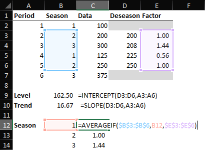
The first argument in the AVERAGEIF function is the season column (B), the second is the season we want to average, and the third is the factor column (E) which is the column that is averaged. I will soon do an Excel in 60 seconds video on this function, follow/subscribe to get notified when it releases.
We now have the average factor for each of the seasons. Now we can move on to forecasting.
Step 4: Forecast
The forecast consists of two parts:
- Forecasting underlying demand
- Applying a seasonal factor
Let’s first add extra rows to forecast another 3 periods (one cycle). Based on our level and trend we can forecast underlying demand.
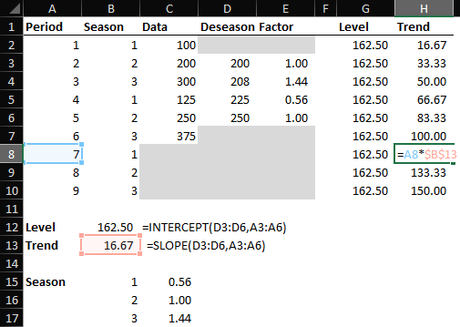
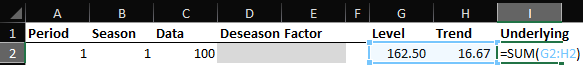
The level is our intercept and does not change. The trend does. Remember that we regressed the deseasonalized data on the periods in Step 2, now we can multiply the trend by the period again. Adding these two together we find the underlying demand.
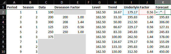
Finally, we apply a seasonal factor. You can use the INDEX or VLOOKUP function to achieve this.
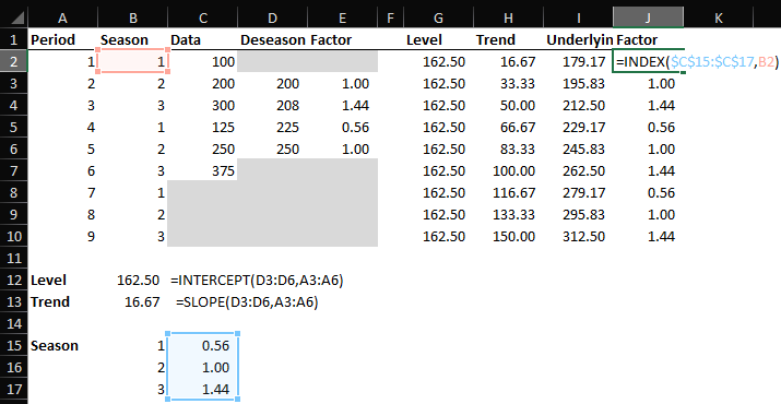
That gives us the average seasonal factor as estimated in Part 4 matching the season for each of the periods.
Finally, we multiply the underlying demand by the seasonal factor to get the Forecast. If you used additive seasonal factors you add the factor instead.
Finally, we can plot our results:
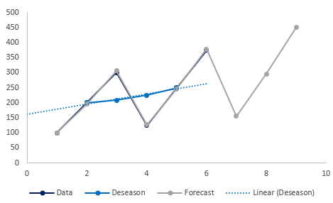
That’s the basics of a static seasonal forecasting model. I’ll leave a good technical chapter below if you’re looking to dig deeper.
Resources:https://host.kelley.iu.edu/mabert/e730/chopra-chap-7.pdf